Generating Multivariate Gaussian Random Numbers
You may have used mvnrnd in Matlab or multivariate_normal in NumPy. How does it work internally? Given a mean vector  and a covariance matrix
  , how would you go about generating a random vector that conforms to a multivariate Gaussian?
While this may sound like a bunch of big words, the intuitive idea behind all of this is: How do I generate numbers that belong the the classic Bell curve shape of the Gaussian. How does it work if I want more than one dimensions? You'll find out in this tutorial.
The roadmap
We know that we can generate uniform random numbers (using the language's built-in random functions). We need to somehow use these to generate n-dimensional gaussian random vectors. We also have a  mean vector and a
  covariance matrix. Here's how we'll do this:
- Generate a bunch of uniform random numbers and convert them into a Gaussian random number with a known mean and standard deviation.
- Do the previous step
 times to generate an n-dimensional Gaussian vector with a known mean and covariance matrix.
 - Transform this random Gaussian vector so that it lines up with the mean and covariance provided by the user.
Generating 1d Gaussian random numbers
We can generate uniform random numbers - for example, rand() / RAND_MAX in C/C++ can be used to generate a number between 0 and 1. Each floating point number between 0 and 1 has equal probability of showing up - thus the uniform randomness. If we want to convert this number into a Gaussian random number, we need to make use of the Central Limit Theorem in probability.
Let's say you generate  uniform random numbers (each between 0 and 1) and you use the variable
  to denote each of these. The Central Limit Theorem allows us to convert these numbers belonging to
  into a single number that belongs to the Guassian distribution
  .
.

Here,  is a one dimensional Gaussian random number - produced using the help of uniform random variables. The
  is derived from the term
  (where
  is the mean of the uniform distribution -
  ). The denominator is derived from the term
  where
where  is the variance of the uniform distribution between 0 and 1 (comes to exactly
  ).
).
As  , we get that
  . Thus, the more uniform random numbers you use, the more accurate the "conversion" to Gaussian would be.
Generating a multivariate Gaussian random number
If we're trying to generate an n-d Gaussian random number, we can run do the previous section times. This would give us numbers that are centered around zero and are independent of each other. This means, the n-d Gaussian random number generated belongs to  . Here
  is an n-dimensional zero vector and
  is a identity matrix (the covariance matrix which describes independent components).
This is the known Gaussian distribution. Now, we need to somehow transform this into the Gaussian distribution described by the mean and covariance matrix supplied by the user.
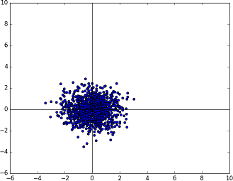
The known multivariate Gaussian distribution in two dimensions N(0, 1)
Linear algebra on the Gaussian distribution
Transforming the Gaussian into the distribution we want is a simple linear transformation. This can be thought of as a two step process. First, we line up the covariance matrix and then we line up the mean.
Lining up the covariance matrix
The Gaussian distribution we have at the moment is perfectly spherical (in n-dimensions) and is centered at the origin. To move towards the Covariance matrix we want, we would need to squash this spherical distribution and maybe rotate it a little bit (to get some correlation).
This can be accomplished by calculating the eigenvectors and eigenvalues of the given covariance matrix and transforming the random number by matrix multiplication.

Here,  is the transformed random number.
  is the diagonal matrix made up of the eigenvalues of and
  is the matrix of eigenvectors (each column is an eigenvector of ).
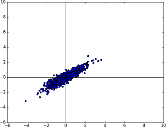
The known multivariate Gaussian distribution now rotated (and squashed) with the help of the given Covariance matrix.
Lining up the mean
At this point, the covariance of the random number is in sync with but we also need to sync up the mean. Luckily, this is very straightforward. The current mean is at the origin - so to have a mean at we simply need to add it.

And this is it. The answer of this equation is a Gaussian random number that belongs to the Gaussian distribution with the desired mean and covariance.
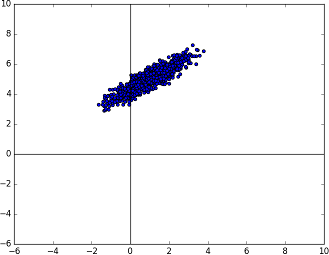
The known multivariate Gaussian distribution now centered at the right mean.
Implementing this with Numpy
Let's start with a new Python script and import the basics:
#!/usr/bin/env python

import numpy as np
import math
import matplotlib.pyplot as plt
We define a function that generates a 1D Gaussian random number for us:
def get_gaussian_random():
    m = 0
    while m == 0:
        m = round(np.random.random() * 100)
It takes no parameters - it returns a Gaussian number with mean 0 and a variance of 1. Here, m refers to the mathematical variable . The higher the value, the more random numbers are used to generate a single Gaussian.
    numbers = np.random.random(int(m))
    summation = float(np.sum(numbers))
    gaussian = (summation - m/2) / math.sqrt(m/12.0)

    return gaussian
These three lines are a bit dense. We use numpy's random number generate to produce m random numbers. We calculate the summation just as mentioned in the Central Limit Theorem. Finally, we put all these numbers together and this produces the Gaussian we were looking for. We return this.
Next, we want to generate several n-dimensional Gaussian random numbers with a zero mean and identity covariance.
def generate_known_gaussian(dimensions):
    count = 1000

    ret = []
    for i in xrange(count):
        current_vector = []
        for j in xrange(dimensions):
            g = get_gaussian_random()
            current_vector.append(g)

        ret.append( tuple(current_vector) )

    return ret
This function simply builds on top of the function we made earlier. It produces count random numbers - each of with has dimensions dimensions. We store each random vector as a tuple and keep appending to a list. Finally, we return the list.
Finally, let's get to the main function:
def main():
    known = generate_known_gaussian(2)
We start out by generating 1000 two dimensional Gaussian random vectors. I chose 2D because they are easier to visualize.
    target_mean = np.matrix([ [1.0], [5.0]])
    target_cov  = np.matrix([[  1.0, 0.7],
                             [  0.7, 0.6]])

    [eigenvalues, eigenvectors] = np.linalg.eig(target_cov)
We define the desired mean and covariance matrix. While we're at it, we also calculate the eigenvalues and eigenvectors of the covariance matrix.
    l = np.matrix(np.diag(np.sqrt(eigenvalues)))
    Q = np.matrix(eigenvectors) * l
Here, we produce the diagonal matrix of eigenvalues ( ) and the temporary matrix Q that stores the matrix multiplication of the eigenvalues and eigenvectors.
    x1_tweaked = []
    x2_tweaked = []
    tweaked_all = []
    for i, j in known:
        original = np.matrix( [[i], [j]]).copy()
Here, I start a loop through all the known random vectors. Since these are 2D vectors, I unpack these into the variables i and j. If you're using a higher dimension, this will not work.
tweaked = (Q * original) + target_mean
I apply the linear transformation: first lining up the covariance and then lining up the mean. And finally:
        x1_tweaked.append(float(tweaked[0]))
        x2_tweaked.append(float(tweaked[1]))
        tweaked_all.append( tweaked )
I save the results in some lists. x1_tweaked holds the transformed first dimension. x2_tweaked holds the second dimension and tweaked_all holds the entire vector.
    plt.scatter(x1_tweaked, x2_tweaked)
    plt.axis([-6, 10, -6, 10])
    plt.hlines(0, -6, 10)
    plt.vlines(0, -6, 10)
    plt.show()

if __name__ == "__main__":
    main()
To close this tutorial, we render out a nice plot that shows the Gaussian distribution of these 1000 points. Here are a few more results and the corresponding covariance matrices (they're all centered at the origin for simplicity):
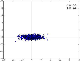
Specimen A with the covariance matrix displayed on the top right corner
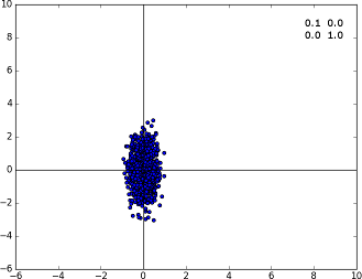
Specimen A with the covariance matrix displayed on the top right corner. Diagonal covariances imply the points are distributed along the axis.
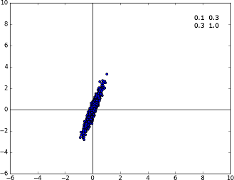
Specimen A with the covariance matrix displayed on the top right corner. When the non-diagonal terms come into action, we see that the distribution rotates a bit.
Numerically verifying the transformation
If you're not satisfied with the math, you may want to learn the mean and covariance of the transformed points and see for yourself. Here's a function that may be of help:
def learn_mean_cov(pts):
    learned_mean = np.matrix([[0.0], [0.0]])
    learned_cov  = np.zeros( (2, 2) )
    count = len(pts)
    for pt in pts:
        learned_mean += pt
        learned_cov  += pt*pt.transpose()

    learned_mean /= count
    learned_cov /= count
    learned_cov -= learned_mean * learned_mean.transpose()

    print(learned_mean)
    print(learned_cov)
In our code, we generated 1000 random vectors. As you increase this count, learned_cov and learned_mean will increasingly move closer to target_cov and target_mean.
Wrap up
I hope you liked this short tutorial. Hopefully this demystified one aspect of scientific computing that you took for granted and helped you appreciate probability a bit more.
Related posts


