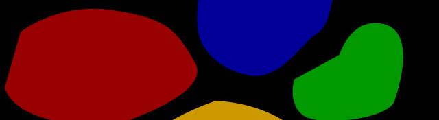
One common problem encountered in image analysis is to figure out which parts of an object are "connected", physically. That is, irrespective of the colour. Here's an example:

In the above image, the red and green circles are distinct. But the goal is not to detect circles (you can do that using the Circle Hough Transform). The goal is to identify the two "blobs". Each blob consisting of two circles, one red and one green.

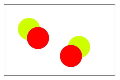
So, the desired output is something like this:

With this type of output, you can easily figure out how many components the image has, and which pixels are connected. The blue pixels are all connected and form one component. Similarly, the green one.

Label

In the current context, labeling is just giving a pixel a particular value. For example, in the previous picture, all pixels in the blue region have the label '1'. Pixels in the green region have the label '2'. The white region, or the background, has the label '0'. This, the problem is to 'label' connected regions in an image.

Another example

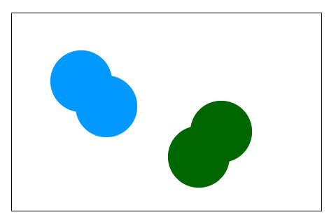
Here's an image generated internally by multitouch applications. The goal is to label each "finger" so that the application can differentiate between the thumb, little finger, etc.

After labeling, the image looks something like this:

Now the application can distinguish between each "finger" very easily.

The recursive algorithm

The recursive algorithm is pretty straightforward. You take a pixel, and check its neighbours for connectivity. But, it's inefficient. As the image size grows, the time taken by the algorithm increases rather quickly. So we won't get into the details of this algorithm.

The classical algorithm

The algorithm designed by Rosenfeld and Pfaltz in 1966 uses the union-find data structure to solve this problem (read about the union-find data structure), and that too quite efficiently. Its "classical" because it uses a result from the the classical algorithm for connectedness in graph theory.

The algorithm consists of two passes. In the first pass, the algorithm goes through each pixel. It checks the pixel above and to the left. And using these pixel's labels (which have already been assigned), it assigns a label to the current pixel. And in the second pass, it cleans up any mess it might have created, like multiple labels for connected regions.

So that was the overview of how the algorithm works. Now we get into the details.

The First Pass

In the first pass, every pixel is checked. One by one, starting at the top left corner, and moving linearly to the bottom right corner.

If you're considering the pixel 'p', you'll only check the orange pixels. Thus, at any given time, you only need to have two rows of the image in memory. This helped in memory efficiency in the past, but now we have 2GB RAMs. So its not an issue these days.

We'll go through each step of the first pass one by one.

Step 1

Here we check if we're interested in a pixel or not. If the pixel is a background pixel (its value is zero, or whatever other criteria you want), we simply ignore it and move on to the next pixel. If not, you go to the next step.

Step 2 and 3

Here, you're fetching the label of the pixels just above and to the left of 'p'. And you store them (into A and B here). Now, there are a few possible cases here:

• The pixel above or/and the the left aren't background pixels: In this case, things proceed as usual. You just go to the next step. A or/and B will have actual values (the labels).
• Both pixels are background pixels: In this case, you cannot get labels. So, you create a new label, and store it into A and B.

Step 4 and 5

You figure out which one is smaller: A or B and then you set that label to pixel 'p'.

Step 6

Suppose you have a situation where pixel above has a label A and the pixel to the left has a label B. But you know that these two labels are connected (because the current pixel "connects them" ).

Thus, you need to store the information that the labels 'A' and 'B' are actually the same. And you do that using the union-find data structure. You set the label 'A' as the child of 'B'. Using this information, the algorithm will clean up the mess in the second mess.

The only thing you need to remember is that the smaller label get assigned to 'p', and the larger number becomes a child of the smaller number.

Step 7

Go to the next pixel.

The second pass

Again, the algorithm goes through each pixel, one by one. It checks the label of the current pixel. If the label is a 'root' in the union-find structure, it goes to the next pixel.

Otherwise, it follows the links to the parent until it reaches the root. Once it reaches the root, it assigns that label to the current pixels.

Done!

That's all there is in this algorithm. You might want to go through the example where I go through each pixel, one by one.