Here we'll be generating the levels histograms you see in Photoshop. You load an image and the R, G and B histograms are calculated and rendered. We'll make a very flexible function which you can reuse in your own projects too.

Loading and splitting the image

First, create a new project. Include the standard OpenCV headers:

#include <stdio.h>
#include <opencv.h>

Next, we get to the main function:

void main()
{

The first thing to do: load an image

    IplImage* img = cvLoadImage("C:\\\\orangeman.jpg");

Next, we create and initialize a histogram:

    int numBins = 256;
    float range[] = {0, 255};

    float *ranges[] = { range };

    CvHistogram *hist = cvCreateHist(1, &numBins, CV_HIST_ARRAY, ranges, 1);
    cvClearHist(hist);

Here, we're creating a uniform 1-D histogram with 256 bins. We supply the range as 0-255. The cvCreateHist function automatically divides this range into 256 bins.

Next, we split the original colour image into its channels. We allocate memory and use the cvSplit function to break it into constituent channels:

    IplImage* imgRed = cvCreateImage(cvGetSize(img), 8, 1);
    IplImage* imgGreen = cvCreateImage(cvGetSize(img), 8, 1);

    IplImage* imgBlue = cvCreateImage(cvGetSize(img), 8, 1);

    cvSplit(img, imgBlue, imgGreen, imgRed, NULL);

The BGR order in the cvSplit command is important. Usually when an image is loaded, this is how its stored in memory.

Rendering histograms

Using the red channel, we can calculate and draw its histogram:

    cvCalcHist(&imgRed, hist, 0, 0);
    IplImage* imgHistRed = DrawHistogram(hist);
    cvClearHist(hist);

The cvCalcHist function calculates the histogram for the image imgRed and stores it into hist. imgHistRed image holds the visual for the histogram. The DrawHistogram function draw it. We'll get to it in a minute.

Finally, we clear the histogram. We're done with the red channel, so we'll reuse it for the green and blue channels too:

    cvCalcHist(&imgGreen, hist, 0, 0);
    IplImage* imgHistGreen = DrawHistogram(hist);

    cvClearHist(hist);

    cvCalcHist(&imgBlue, hist, 0, 0);
    IplImage* imgHistBlue = DrawHistogram(hist);
    cvClearHist(hist);

Then we display these histograms in their own little windows:

    cvNamedWindow("Red");
    cvNamedWindow("Green");

    cvNamedWindow("Blue");

    cvShowImage("Red", imgHistRed);
    cvShowImage("Green", imgHistGreen);

    cvShowImage("Blue", imgHistBlue);

    cvWaitKey(0);
}

The cvWaitKey ensures that the windows don't close automatically. You need to press a key to continue. With that, the main function is done. Now we'll create the DrawHistogram function.

A function to draw histograms

Begin by defining the parameters:

IplImage* DrawHistogram(CvHistogram *hist, float scaleX=1, float scaleY=1) 
{

The function takes one histgoram (that it needs to render) and the scale on the X and Y axes. By default the histogram size is 256x64. Using the scale factors, you can get whatever size you want.

The values in the histogram can be extremely varied. From values less than 0.1 to greater than 1000. We need to fit all these into an image with a finite number of pixels.

So we figure out the maximum value of the histogram. Using this maximum, we scale the other values so they fit into the vertical size of the image:

    float histMax = 0;
    cvGetMinMaxHistValue(hist, 0, &histMax, 0, 0);

Next, we create and blank out an image of the desired size:

    IplImage* imgHist = cvCreateImage(cvSize(256*scaleX, 64*scaleY), 8 ,1);
    cvZero(imgHist);

Then, we go through all bins and render out the graphic:

    for(int i=0;i<255;i++)
    {
        float histValue = cvQueryHistValue_1D(hist, i);

        float nextValue = cvQueryHistValue_1D(hist, i+1);

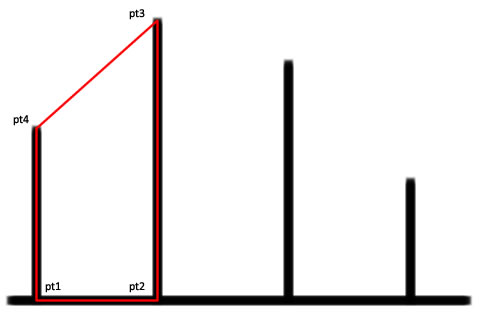
        CvPoint pt1 = cvPoint(i*scaleX, 64*scaleY);
        CvPoint pt2 = cvPoint(i*scaleX+scaleX, 64*scaleY);
        CvPoint pt3 = cvPoint(i*scaleX+scaleX, (64-nextValue*64/histMax)*scaleY);

        CvPoint pt4 = cvPoint(i*scaleX, (64-histValue*64/histMax)*scaleY);

        int numPts = 5;

        CvPoint pts[] = {pt1, pt2, pt3, pt4, pt1};

        cvFillConvexPoly(imgHist, pts, numPts, cvScalar(255));
    }

Finally, we return the image we created:

    return imgHist;
}

Two things to remember with this function.

• You're allocating memory in the function. So no need to do it anywhere else
• Since the memory is allocated withing the image and not released, you must ensure it gets released when its work is done

How the rendering works?

To draw the histogram, the cvFillConvexPoly function is used. This function can draw filled polygons. You pass the array of points and the number of points along with the color and it does its job.

The points pt1...pt4 are calculated and this polygon is rendered using the cvFillConvexPoly function. This is done for every single bin.

This polygon method produces relatively better results than simply drawing a straight vertical line at the center of a bin. If you did  the latter, you'd get a result like the black part. With the polygon method, values "in-between" get rendered as well.

Summary

With this post, you have a handy function that you can use to render out any 1D histogram. Just make sure it is 1D and not a sparse histogram. I haven't added any checks for that.