
Convolutions
Image convolution examples
Series: Convolutions:
- Basics of convolutions
- Image convolution examples
A convolution is very useful for signal processing in general. There is a lot of complex mathematical theory available for convolutions. For digital image processing, you don't have to understand all of that. You can use a simple matrix as an image convolution kernel and do some interesting things!
Simple box blur
Here's a first and simplest. This convolution kernel has an averaging effect. So you end up with a slight blur. The image convolution kernel is:
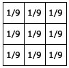
Note that the sum of all elements of this matrix is 1.0. This is important. If the sum is not exactly one, the resultant image will be brighter or darker.
Here's a blur that I got on an image:
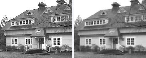
A simple blur done with convolutions
Gaussian blur
Gaussian blur has certain mathematical properties that makes it important for computer vision. And you can approximate it with an image convolution. The image convolution kernel for a Gaussian blur is:
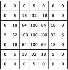
Here's a result that I got:
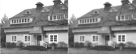
Line detection with image convolutions
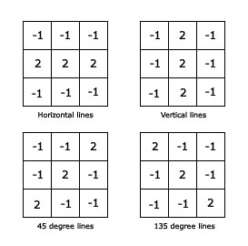
With image convolutions, you can easily detect lines. Here are four convolutions to detect horizontal, vertical and lines at 45 degrees:
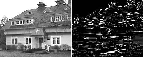
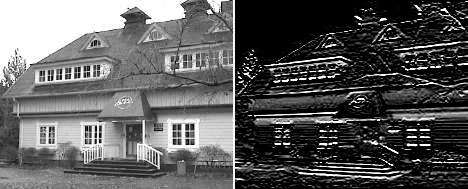
 I looked for horizontal lines on the house image. The result I got for this image convolution was:
Edge detection
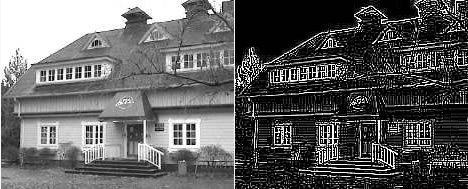
The above kernels are in a way edge detectors. Only thing is that they have separate components for horizontal and vertical lines. A way to "combine" the results is to merge the convolution kernels. The new image convolution kernel looks like this:

Below result I got with edge detection:
The Sobel Edge Operator
The above operators are very prone to noise. The Sobel edge operators have a smoothing effect, so they're less affected to noise. Again, there's a horizontal component and a vertical component.
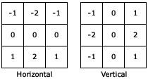
On applying this image convolution, the result was:
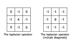
The laplacian operator
The laplacian is the second derivative of the image. It is extremely sensitive to noise, so it isn't used as much as other operators. Unless, of course you have specific requirements.
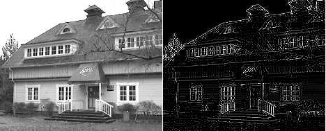
Here's the result with the convolution kernel without diagonals:
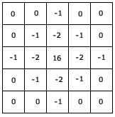
The Laplacian of Gaussian
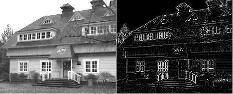
The laplacian alone has the disadvantage of being extremely sensitive to noise. So, smoothing the image before a laplacian improves the results we get. This is done with a 5x5 image convolution kernel.
The result on applying this image convolution was:
Summary
You got to know about some important operations that can be approximated using an image convolution. You learned the exact convolution kernels used and also saw an example of how each operator modifies an image. I hope this helped!
More in the series
This tutorial is part of a series called Convolutions:
- Basics of convolutions
- Image convolution examples


