Convolutions is a technique for general signal processing. People studying electrical/electronics will tell you the near infinite sleepless nights these convolutions have given them. Entire books have been written on this topic. And the questions and theorems that need to be proved are [insurmountable]. But for computer vision, we'll just deal with some simple things.

The Kernel

A convolution lets you do many things, like calculate derivatives, detect edges, apply blurs, etc. A very wide variety of things. And all of this is done with a "convolution kernel".

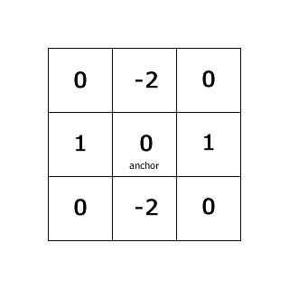
The convolution kernel is a small matrix. This matrix has numbers in each cell and has an anchor point:

This kernel slides over an image and does its thing. The "anchor" point is used to determine the position of the kernel with respect to the image.

The transformation

The anchor point starts at the top-left corner of the image and moves over each pixel sequentially. At each position, the kernel overlaps a few pixels on the image. Each overlapping pair of numbers is multiplied and added. Finally, the value at the current position is set to this sum.

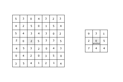
Here's an example:

The matrix on the left is the image and the one on the right is the kernel. Suppose the kernel is at the highlighted position. So the '9' of the kernel overlaps with the '4' of the image. So you calculate their product: 36. Next, '3' of the kernel overlaps the '3' of the image. So you multiply: 9. Then you add it to 36. So you get a sum of 36+9=45. Similarly, you do for all the remaining 7 overlapping values. You'll get a total sum. This sum is stored in place of '2' (in the image).

Speed optimizations

The most direct way to compute a convolution would be to use multiple for loops. But that causes a lot of repeated calculations. And as the size of the image and kernel increases, the time to compute the convolution increases too (quite drastically).

Techniques haves been developed to calculate convolutions rapidly. One such technique is using the Discrete Fourier Transform. It converts the entire convolution operation into a simple multiplication. Fortunately, you don't need to know the math to do this in OpenCV. It automatically decides whether to do it in frequency domain (after the DFT) or not.

Problematic corners and edges

The kernel is two dimensional. So you have problems when the kernel is near the edges or corners. Here's an example: If the kernel (in the above example) is on the top right position, the '0' of the kernel will be over the '3' in the image. But the '1' will be outside the image. So we have no idea what to do with it. Two things are possible:

• Ignore the ones -or-
• Do something about the edges Usually people choose to do something about it. They create extra pixels near the edges. There are a few ways to create extra pixels:
• Set a constant value for these pixels
• Duplicate edge pixels
• Reflect edges (like a mirror effect)
• Warp the image around (copy pixels from the other end)

This usually fixes the problems that might arise.

Summary

You learned a powerful technique that can be used for a lot of different purposes. We'll see a few of those next.