
Cropping robotics arena boundaries: Implementation
In the previous article, Cropping robotics arena boundaries, I talked about the steps involved in getting rid of everything beyond the arena boundary. In this article, I'll go into the coding aspects. We'll start by loading the image into memory, and then go through each step in detail. By the end, you'll have a working program that crops the arena awesomely :P! I'll be using OpenCV for the image processing part. Though I'm sure OpenCV specific commands should have equivalents in other image processing libraries as well.
Juggling code
I assume you have OpenCV install (check OpenCV 2.0 on Windows or the more detailed Installing and getting OpenCV running). I'll be using Visual Studio 2008 for this project. But it should translate without many changes for other IDE's as well.
Start Visual Studio and create a new project. Choose Visual C++ > Win32 > Win32 Console Application as the project type and name it whatever you want. Click OK and then accept all default settings by clicking Finish.
You'll have a blank skeleton project ready. We'll start by including the main OpenCV headers
// ArenaCrop.cpp : Defines the entry point for the console application.
//
#include "stdafx.h"
Just below the stdafx.h line, add these lines:
#include <cv.h>
#include <highgui.h>
#include <math.h>
We've included OpenCV's headers and mathematical functions as well. Next, we get to the main() function:
int main()
{
The first thing to do is get the image of the arena, and save its size in a variable:
int main()
{
    IplImage* img = cvLoadImage("C:\\\\goal_arena.jpg");
    CvSize imgSize = cvGetSize(img);
Now we'll create several other images that we'll be using during the processing:
    IplImage* detected = cvCreateImage(imgSize, 8, 1);

    IplImage* imgBlue = cvCreateImage(imgSize, 8, 1);
    IplImage* imgGreen = cvCreateImage(imgSize, 8, 1);
    IplImage* imgRed = cvCreateImage(imgSize, 8, 1);
detected will store the "white" parts of the arena. And the images imgBlue, imgGreen and imgRed hold the three channels of the arena. Note that all these images are single channel images.
The cvSplit function will separate the loaded image (img) into its channels and store them in the three parameters given.
cvSplit(img, imgBlue, imgGreen, imgRed, NULL);
With individual channels, we can easily detect the white parts of the image like this:
    cvAnd(imgGreen, imgBlue, detected);
    cvAnd(detected, imgRed, detected);
This ANDs the first two parameters and stores it in the third parameter. The results from this aren't great. There are lots of unwanted pixels that make it through. Here's a picture of whats stored in detected after the ANDing is done:
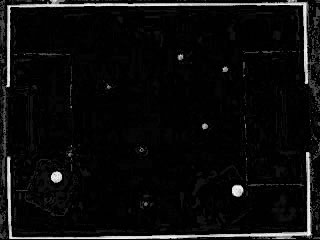
We need to get rid of all that noise. So, we open the image (morphological opening) and then threshold detected.
    cvErode(detected, detected);
    cvDilate(detected, detected);    // Opening

    cvThreshold(detected, detected, 100, 250, CV_THRESH_BINARY);
Opening is an erosion followed by a dilation. And you can read about thresholding, its just keeping pixels above a certain value, and trashing the rest. Here's what it looks like after this is done:
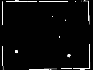
Now we get to the juice of the tutorial. We'll use an inbuilt function to do a hough transform on detected and get a list of lines:
    CvMat* lines = cvCreateMat(100, 1, CV_32FC2);
    cvHoughLines2(detected, lines, CV_HOUGH_STANDARD, 1, 0.001, 100);
The lines matrix is a two channeled, floating matrix with 100 rows and 1 column. We'll store the parameters returned by the hough transform (the p and θ of the lines in normal form) in this matrix. And we cannot store more than 100 lines in the matrix. This might vary in your case. I use a 320x240 image, so it works fine for me. If you use a bigger image (1280x720 :O ) then you might need a lot more rows in the matrix.
The function cvHoughLines2 actually the hough transform on detected and stores the results in lines. CV_HOUGH_STANDARD ensures that the function does the classical hough transform. The classical hough transform returns lines instead of line segments. If you check the result we get after thresholding, you'll see we have short line segments. But we're interested in infinite lines. So we choose the standard hough transform.
The 1 and 0.001 are the accuracy of the values of p and θ respectively. p is in pixels, so we set it to 1. θ is in radians, which is extremely sensitive. So we set its accuracy to 0.001. You can increase precision if you want, but that would increase run time.
The 100 is a kind of selection criteria. If a line gets a score of greater than 100, the function adds it to lines. Otherwise, the line is assumed to be part of noise and ignored. Read more about The Hough Transform and you'll get to know what this is.
Once the hough transform is done, we're ready to sort through the list of lines we get.
How to sort through lines
Before we get to the code that does this, let me explain how we'll go about doing that. For each ;line, the matrix has two parameters (p and θ). Based on their values, we can roughly estimate if it is a top boundary, a left boundary, a right boundary or a bottom boundary. How do you do that? Here's how:
Always, the top left point is (0, 0). So that's the origin. The parameter values are relative to this point:
- p > image's height/2 AND θ is around 0 degrees: this line is a right boundary
- p > image's height/2 AND θ is around 90 degrees: this line is a bottom boundary
- p < image's height/2 AND θ is around 0 degrees: this line is a top boundary
- p < image's height/2 AND θ is around 90 degrees: this line is a left boundary
These pictures should explain you why the above conditions hold:

The red line has been returned by the hough transform. You can see the θ is almost zero, and p is quite long. So we can conclude this particular line belongs to the right edge. Try figuring out the conditions for the other boundaries yourself:

The next important thing we need to do is merge several lines. Why? The "lines" in the thresholded image are thick. So the hough transform might return several lines for every boundary. So we need a "mechanism" to calculate a single line from all those lines.
This is done by averaging two points of the lines. Again, a graphic should serve to explain the idea better:

All the red lines have been categorized as at belonging near the top edge. So, summing the x and y coordinates and dividing by the number of points, we get the averaged top edge... represented by the black line.
With these two ideas, we're ready to proceed with coding!
Back to coding
Okay, so where were we?
We had called cvHoughLines2 and now we need to sort the lines, and generate single boundary lines. We've written code till here:
    CvMat* lines = cvCreateMat(100, 1, CV_32FC2);
    cvHoughLines2(detected, lines, CV_HOUGH_STANDARD, 1, 0.001, 100);
The next thing we do is, declare several variables:
    CvPoint left1 = cvPoint(0, 0);
    CvPoint left2 = cvPoint(0, 0);
    CvPoint right1 = cvPoint(0, 0);
    CvPoint right2 = cvPoint(0, 0);
    CvPoint top1 = cvPoint(0, 0);
    CvPoint top2 = cvPoint(0, 0);
    CvPoint bottom1 = cvPoint(0, 0);

    CvPoint bottom2 = cvPoint(0, 0);

    int numLines = lines->rows;
    int numTop = 0;
    int numBottom = 0;
    int numLeft = 0;
    int numRight = 0;
We're creating variables to hold the endpoints of the lines for the averaging thingy. numLines _stores the number of lines, and _numTop, numBottom, _numLeft _and _numRight _store the number of lines for each edge (yes, each boundary can have different number of lines)
Next we look at each line:
    for(int i=0;i<numLines;i++)
    {
And we get the two parameters for the current line:
        CvScalar dat = cvGet1D(lines, i);
        double rho = dat.val[0];
        double theta = dat.val[1];
The value of rho is in pixels, and theta is in radians. If theta is zero, it means the line is exactly vertical. This causes some problems with the averaging process (infinites). So we simply ignore these lines:
        if(theta==0.0)
            continue;
If not, we can approximate this line. So we convert the angle from radians to degrees, and generate two points on the line.
        double degrees = theta*180/(3.1412);

        CvPoint pt1 = cvPoint(0, rho/sin(theta));
        CvPoint pt2 = cvPoint(img->width, (-img->width/tan(theta)) + rho/sin(theta));
We generate the two points by using the normal-form equation of line:
p = x*cosθ + y*sinθ
We know p and θ, and we want to generate two x's and y's. We do that by setting x=0 and x=image's width, and then calculating the value of y.
Now, we get to the "categorization part. We'll figure out which edge the line is closest too. And do the averaging thingy there itself.
        if(abs(rho)<50)
        {
We check if the absolute value of rho is less than 50. If it is, the current line is either the top edge or the left edge. We figure this out using a condition on the angle:
            if(degrees>45 && degrees<135)
            {
If the angle is around 90 degrees, it's the top edge. So we sum up the two points we generated into top1 and top2.
                numTop++;

                // The line is vertical and near the top
                top1.x+=pt1.x;

                top1.y+=pt1.y;

                top2.x+=pt2.x;
                top2.y+=pt2.y;
            }
Otherwise, the line is a left edge:
            else
            {

                numLeft++;

                // The line is vertical and near the left
                left1.x+=pt1.x;

                left1.y+=pt1.y;

                left2.x+=pt2.x;
                left2.y+=pt2.y;
            }
        }
If the absolute of rho is not less than 50, it has to be either the right edge of the bottom edge.
        else
        {
            // We're in the right portion
            if(degrees>45 && degrees<135)
            {

                numBottom++;

                //The line is horizontal and near the bottom
                bottom1.x+=pt1.x;

                bottom1.y+=pt1.y;

                bottom2.x+=pt2.x;
                bottom2.y+=pt2.y;
            }
            else
            {

                numRight++;

                // The line is vertical and near the right
                right1.x+=pt1.x;

                right1.y+=pt1.y;

                right2.x+=pt2.x;
                right2.y+=pt2.y;
            }
        }
    }
Well, up till now we've just added the x and y coordinates. Now is the time to divide them by the number of points.
    left1.x/=numLeft;
    left1.y/=numLeft;
    left2.x/=numLeft;

    left2.y/=numLeft;

    right1.x/=numRight;
    right1.y/=numRight;
    right2.x/=numRight;

    right2.y/=numRight;

    top1.x/=numTop;
    top1.y/=numTop;
    top2.x/=numTop;

    top2.y/=numTop;

    bottom1.x/=numBottom;
    bottom1.y/=numBottom;
    bottom2.x/=numBottom;
    bottom2.y/=numBottom;
You see we can't just divide each by numLines/4. Each boundary has a different number of lines. After the division, we have two points on a single line for each edge! You can draw these lines onto the original image (img):
    cvLine(img, left1, left2, CV_RGB(255, 0,0), 1);
    cvLine(img, right1, right2, CV_RGB(255, 0,0), 1);
    cvLine(img, top1, top2, CV_RGB(255, 0,0), 1);

    cvLine(img, bottom1, bottom2, CV_RGB(255, 0,0), 1);
After this, img looks something like this:
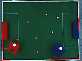
Now, we solve for intersection of these lines. I won't go into the details here (this article has already turned massive). Thought, you might want to read about solving for intersection of lines. Here's the entire code that does it:
    // Next, we need to figure out the four intersection points
    double leftA = left2.y-left1.y;
    double leftB = left1.x-left2.x;

    double leftC = leftA*left1.x + leftB*left1.y;

    double rightA = right2.y-right1.y;
    double rightB = right1.x-right2.x;

    double rightC = rightA*right1.x + rightB*right1.y;

    double topA = top2.y-top1.y;
    double topB = top1.x-top2.x;

    double topC = topA*top1.x + topB*top1.y;

    double bottomA = bottom2.y-bottom1.y;
    double bottomB = bottom1.x-bottom2.x;

    double bottomC = bottomA*bottom1.x + bottomB*bottom1.y;

    // Intersection of left and top
    double detTopLeft = leftA*topB - leftB*topA;

    CvPoint ptTopLeft = cvPoint((topB*leftC - leftB*topC)/detTopLeft, (leftA*topC - topA*leftC)/detTopLeft);

    // Intersection of top and right
    double detTopRight = rightA*topB - rightB*topA;

    CvPoint ptTopRight = cvPoint((topB*rightC-rightB*topC)/detTopRight, (rightA*topC-topA*rightC)/detTopRight);

    // Intersection of right and bottom
    double detBottomRight = rightA*bottomB - rightB*bottomA;

    CvPoint ptBottomRight = cvPoint((bottomB*rightC-rightB*bottomC)/detBottomRight, (rightA*bottomC-bottomA*rightC)/detBottomRight);

    // Intersection of bottom and left
    double detBottomLeft = leftA*bottomB-leftB*bottomA;
    CvPoint ptBottomLeft = cvPoint((bottomB*leftC-leftB*bottomC)/detBottomLeft, (leftA*bottomC-bottomA*leftC)/detBottomLeft);
The basic idea is to solve the two line equations simultaneously. In the article on Solving for intersection of lines I talk about A, B and C. We calculate these constants for each line (topA, topB, topC, etc) and then use those to determine the intersection points.
The intersections are stored in ptTopLeft, ptTopRight, ptBottomRight _and _ptBottomLeft. You can render the intersections on the original image:
    cvLine(img, ptTopLeft, ptTopLeft, CV_RGB(0,255,0), 5);
    cvLine(img, ptTopRight, ptTopRight, CV_RGB(0,255,0), 5);
    cvLine(img, ptBottomRight, ptBottomRight, CV_RGB(0,255,0), 5);
    cvLine(img, ptBottomLeft, ptBottomLeft, CV_RGB(0,255,0), 5);
This adds green points at the corners of the arena.
Now we're ready to generate the actual mask. To do this, we create a new image:
    IplImage* imgMask = cvCreateImage(imgSize, 8, 3);
    cvZero(imgMask);
The cvZero ensures that the entire image is completely black. Next, we use the cvFillConvexPoly command to create a filled polygon with the corner points we just found.
    CvPoint* pts = new CvPoint[4];
    pts[0] = ptTopLeft;
    pts[1] = ptTopRight;
    pts[2] = ptBottomRight;
    pts[3] = ptBottomLeft;
    cvFillConvexPoly(imgMask, pts, 4, cvScalar(255,255,255));
This command expects an array of points. So we had to create one. This function takes 4 parameters. The first is the image to draw to (imgMask in this case). pts is the actual array of points. You also need to supply the number of points (in this case, 4). And finally, the color to fill with.
After doing this, you'll get a mask that looks something like this:
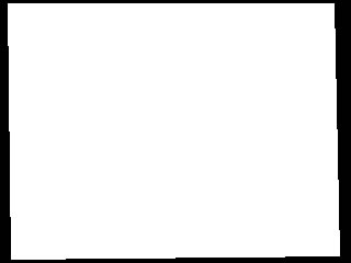
We'll do the final touch:
    cvAnd(img, imgMask, img);

    cvNamedWindow("Original");

    cvNamedWindow("Detected");

    cvShowImage("Original", img);
    cvShowImage("Detected", detected);

    cvWaitKey(0);

    return 0;
}
The AND imposes the mask onto the original image. Thus, eliminating anything that's outside the arena boundary.
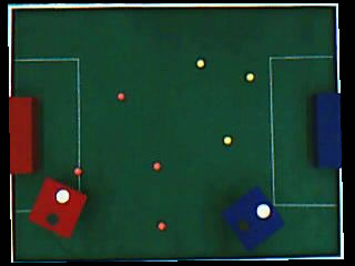
That's a pretty good result in my opinion. The lines don't have to perfectly straight, or parallel to the edges. They might even curve a bit. Even then the algorithm will work. Interesting!
Done!
And there you have it. How it's done. In extreme detail. This was one HUGE articles... it's around 2200 words. Massive. I hope you liked it, and learned a bit as well.


