Models?! Where?!?!!

Technically, it is possible to "represent" random noise as a mathematical function. And that is exactly what a model is. The "distribution" of noise is based on probability. Hence the model is called a Probability Density Function (PDF).

Once noise has been quantified, creating filters to get rid of it becomes a lot more easier. In this article, we'll just be going through the various PDFs (probability density functions) and get acquainted with six different noise models.

Probability Density Functions (PDF)

Okay, the name sound scary. Terrifying maybe. But PDFs are simple once you understand their real meaning. Right now, I'll just try and explain the concept...

Consider the distribution of numbers below (I just made it up in 2 minutes):

In this graph, the vectical axis represents probability. And the horizontal axis represents numbers.

Now here's the thing: The probability a randomly picked number (say x) lies in a range from a to b (a,b) is equal to the area of the curve between a and b.

If you take infinite random numbers, distributed as shown above, then:

• If you pick a number randomly, then there is a 0% chance that it will be a 49. That's because the "area" between 49 and 49 is, well, zero.
• Similarly, there is a 75% chance that the number will be -73 or 49. Thats because a lot of area under the curve is between -73 and 49.
• There is a 100% chance of picking a number between +infinity or -infinity

These hold because the PDF satisfies some conditions. You could take an entire course at your university if you want to get into the mathematical details. So I won't go into the details here.

There are certain mathematical properties of the distribution as well: the mean and the variance.

The mean is roughly the "middle value" of the entire distribution. In the distribution above, the mean would be slightly shifted to the left (because of its skewed nature).

The variance is a measure of how much the probabilities vary. A greater variance means you're more likely several different values. A smaller variance means you'll get lesser different values. Have a look at these two PDFs:

The one on the left is "broader". So you'll end up getting lots of -73s and 49s. But the one on the right isn't. You won't end up with lots of -73s and 49s. I hope you get an idea.

Mathematics of PDFs allows you to precisely calculate the value of the mean and variance. But again, we won't go into all those details. Just these ideas are enough for us to build upon our image processing and computer vision knowledge

The Gaussian Noise Distribution

The figure above shows two gaussian PDFs. Now, if they represent noise, what would it mean?

Considering the blue PDF: the mean value of the noise will be -2. So, on an average, 2 would be subtracted from all pixels of the image. You'll also have 7 being subtracted... or even 3 being added as noise. This is because the distribution extends of a broad range of values.

In the red PDF, the mean value is 3. So on an average, 3 would be added to all pixels. You'll see some pixels having 1 added or 5 added. But because the distribution isn't that wide, you'll see a narrow variation in noise.

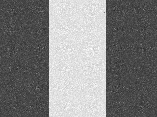
Example:

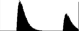
Above: The original image. Below: The image with gaussian noise. The histogram for each of these images is:

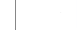
The upper image is the histogram for the original image. Because it has only 2 colours, there are just two spikes.

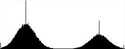
The lower image is the histogram for noisy image. When noise is added, notice how "gaussian-like" the histogram becomes. Each spike in the original image "turns" into something similar to a gaussian distribution. That is exactly the reason why it is called gaussian noise. It usually occurs in an image due to noise in electronic circuits and noise in the sensor itself (maybe due to poor illumination or at times even high temperature).

Also, this type of noise is called Independent noise. Thats because the noise does not have any relation with the actual image data. It just occurs randomly.

The Gamma Noise Distribution

Just like gaussian, the Gamma distribution has a distinct PDF. Here it is:

Applying gamma noise to an image produces the following results:

Again, here are the histograms:

Again, adding gamma noise "turns" the spike into a gamma distribution like thingy. Also, this is independent noise.

Next, we'll see 2 similar noise distributions, one completely different noise distribution (the salt and pepper noise) and also the unique uniform noise distribution.