The Exponential Noise Distribution

The exponential distribution distribution looks like this:

Here's a sample of what exponential noise looks like:

The histograms for the above images are:

Again, you see something similar to the exponential distribution. This is also independent noise and is used to model noise in laser imaging.

The Rayleigh Noise Distribution

Here's the characteristic plot of the Rayleigh probability distribtion function:

And here's what rayleigh noise looks like:

And here's the histograms for both of the images above:

This too is independent noise and is used to characterize noise in range imaging.

The Uniform Noise Distribution

Now for something new. Instead of all the curvy graphs till now, the uniform distribution has a flat line. It looks like this:

Here, all the values between a and b have an equal probability of occuring. Hence the flat top. Here's what uniform noise looks like:

And, as usual, here are the histograms for them:

Looks pretty "uniform" right? This, too, is independent noise. This noise model doesn't resemble any practical situation. Its there just because computers always generate uniform random numbers. So generating uniform noise isn't tough.

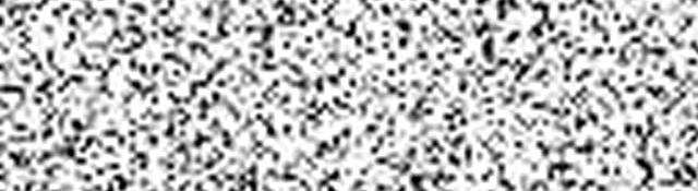
The Impulse Noise Distribution: Salt and Pepper Noise

Here's something completely new. No probability distribution function here. Have a look at the following images:

You'd have noticed that this noise looks very different from the ones we've seen earlier. You can simply visually distinguish between this noise and the others we've discussed so far.

Its called salt and pepper because it looks like that: the white specks are the salt, the black ones are the pepper.

This noise is generally produced when transmitting an image. The value of the pixel just gets corrupted: all bits of the pixel turn into a 1, or into a 0... or the bits invert (1 turns into a 0, and vice versa).

Representing this mathematically is a bit complicated. And generally, this is a Data dependent noise.

Here are the histograms for the two images just shown:

Notice how the original spikes remain preserved. Only little spikes are added at the very extremities of the histogram. The leftmost little spike being for the "pepper" and the right most being for the "salt".

Conclusion

So we discussed 6 unique noise distributions in this article. Now you're in direct competition with Photoshop... which just offers Gaussian and Uniform noise! Go defeat some photoshop with OpenCV!

And, I've created a little program that lets you generate all these noises in realtime. Feel free to download and experiment with it. You can choose between different noise types by pressing the keys 1-6. You can download it from the link below.